Python for Finance Chapter1

I started to study the book of Python for Finance. With the previous foundation of python and the knowledge of financial numerical calculation, I think it should not be too difficult. Fighting! ! !

Part I. Python and Finance

This part introduces Python for finance. It consists of two chapters:

• Chapter 1 discusses Python in general and argues in some detail why Python is well suited to addressing the technological challenges in the financial industry as well as in financial data analytics.

• Chapter 2 is about Python infrastructure; it provides a concise overview of important aspects of managing a Python environment to get you started with interactive financial analytics and financial application development in Python.

Chapter 1. Why Python for Finance

Introduce Python balabala…

Python itself already comes with a large set of packages and modules that enhance the basic interpreter in different directions, known as the Python Standard Library. For example, basic mathematical calculations can be done without any importing, while more specialized mathematical functions need to be imported through the math module

1
2
3
4
5
6
7
8
9
10
11
12
13
14
15
16
17

ln[1]:100 * 2.5 + 50

		300.0

ln[2]:log(1) 

        ---------------------------------------------------------------------------
        NameError                                 Traceback (most recent call last)
        <ipython-input-2-78aa16009595> in <module>
        ----> 1 log(1)

        NameError: name 'log' is not defined

ln[3]:import math
	  math.log(1)

		0.0

• Without further imports, an error is raised.

• After importing the math module, the calculation can be executed.

The Scientific Stack

There is a certain set of packages that is collectively labeled the scientific stack. This stack comprises, among others, the following packages:

NumPy

NumPy provides a multidimensional array object to store homogeneous or heterogeneous data; it also provides optimized functions/methods to operate on this array object.

SciPy

SciPy is a collection of subpackages and functions implementing important standard functionality often needed in science or finance; for example, one finds functions for cubic splines interpolation as well as for numerical integration.

matplotlib

This is the most popular plotting and visualization package for Python, providing both 2D and 3D visualization capabilities.

pandas

pandas builds on NumPy and provides richer classes for the management and analysis of time series and tabular data; it is tightly integrated with matplotlib for plotting and PyTables for data storage and retrieval.

scikit-learn

scikit-learn is a popular machine learning (ML) package that provides a unified application programming interface (API) for many different ML algorithms, such as for estimation, classification, or clustering.

PyTables

PyTables is a popular wrapper for the HDF5 data storage package; it is a package to implement optimized, disk-based I/O operations based on a hierarchical database/file format.

Technology in Finance

…

Python for Finance

Finance and Python Syntax

Most people who make their first steps with Python in a finance context may attack an algorithmic problem. This is similar to a scientist who, for example, wants to solve a differential equation, evaluate an integral, or simply visualize some data. In general, at this stage, little thought is given to topics like a formal development process, testing, documentation, or deployment. However, this especially seems to be the stage where people fall in love with Python. A major reason for this might be that Python syntax is generally quite close to the mathematical syntax used to describe scientific problems or financial algorithms.（我就是最近这样迷上python的）

This can be illustrated by a financial algorithm, namely the valuation of a European call option by Monte Carlo simulation.(一个蒙特卡罗计算欧式期权定价的例子)

• Initial stock index level S0 = 100 （股票初始价格）
• Strike price of the European call option K = 105 （期权的执行价格）
• Time to maturity T = 1 year （到期时间）
• Constant, riskless short rate r = 0.05 （固定的无风险利率）
• Constant volatility σσ = 0.2 （固定的波动率）

In the BSM model, the index level at maturity is a random variable given by BSM Equation below, with z being a standard normally distributed random variable.

Black-Scholes-Merton (1973) Equation:
$$
S_T = S_0exp((r-\frac{1}{2}\sigma^2)T+\sigma\sqrt{T}z))
$$
The following is an algorithmic description of the Monte Carlo valuation procedure:

1. Draw I pseudo-random numbers $Z(i),i \in {1,2,\dots,I}$, from the standard normal distribution.
2. Calculate all resulting index levels at maturity $S_T(i)$ for given $z(i)$ and Equation above.
3. Calculate all inner values of the option at maturity as $h_T(i)=max(S_T(i)-k,0)$.
4. Estimate the option present value via the Monte Carlo estimator as given in Equation blow.

Monte Carlo estimator for European option:
$$
C_0 \approx e^{-rT}\frac{1}{I}\sum_{I}h_T(i)
$$
This problem and algorithm must now be translated into Python. The following code implements the required steps:

1
2
3
4
5
6
7
8
9
10
11
12
13
14
15
16
17
18

import math
import numpy as np

S0 = 100. 
K = 105.
T = 1.0  
r = 0.05  
sigma = 0.2  

I = 100000  
np.random.seed(1000)  
z = np.random.standard_normal(I)  
ST = S0 * np.exp((r - sigma ** 2 / 2) * T + sigma * math.sqrt(T) * z) 
hT = np.maximum(ST - K, 0) 
C0 = math.exp(-r * T) * np.mean(hT)  

print('Value of the European call option: {:5.3f}.'.format(C0)) 
         Value of the European call option: 8.019.

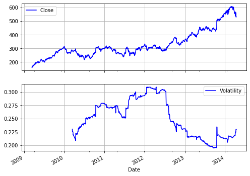
Consider a finance student who is writing their master’s thesis and is interested in S&P 500 index values. They want to analyze historical index levels for, say, a few years to see how the volatility of the index has fluctuated over time and hope to find evidence that volatility, in contrast to some typical model assumptions, fluctuates over time and is far from being constant. The results should also be visualized. The student mainly has to do the following:

• Retrieve index level data from the web
• Calculate the annualized rolling standard deviation of the log returns (volatility)
• Plot the index level data and the volatility results

1
2
3
4
5
6
7
8

import numpy as np
import pandas as pd
import pandas_datareader.data as web

goog = web.DataReader('GOOG', data_source='yahoo',
                      start='3/14/2009', end='4/14/2014')
goog.index.name = 'Date'
goog.tail()

out:

• Volatility

1
2
3
4
5
6
7

goog['Log_Ret'] = np.log(goog['Close'] / goog['Close'].shift(1))
# goog['Volatility'] = pd.rolling_std(goog['Log_Ret'], window=252) * np.sqrt(252)
goog['Volatility'] = goog['Log_Ret'].rolling(252).std() * np.sqrt(252)

%matplotlib inline
goog[['Close', 'Volatility']].plot(subplots=True, color='blue',
                                   figsize=(8, 6), grid=True);

PERFORMANCE COMPUTING WITH PYTHON

1
2
3
4
5
6

loops = 25000
from math import *
a = range(1, loops)
def f(x):
    return 3 * log(x) + cos(x) ** 2
%timeit r = [f(x) for x in a]

14.4 ms ± 211 µs per loop (mean ± std. dev. of 7 runs, 100 loops each)

1
2
3

import numpy as np
a = np.arange(1, loops)
%timeit r = 3 * np.log(a) + np.cos(a) ** 2

377 µs ± 225 ns per loop (mean ± std. dev. of 7 runs, 1000 loops each)

Using NumPy considerably reduces the execution time to about 88 milliseconds. However, there is even a package specifically dedicated to this kind of task. It is called numexpr, for “numerical expressions.” It compiles the expression to improve upon the performance of the general NumPy functionality by, for example, avoiding in-memory copies of ndarray objects along the way:(使用 numexpr 库编译表达式，改善 numpy 的性能，例如在执行期间避免数组在内存中的复制)

1
2
3
4

import numexpr as ne
ne.set_num_threads(1)
f = '3 * log(a) + cos(a) ** 2'
%timeit r = ne.evaluate(f)

232 µs ± 201 ns per loop (mean ± std. dev. of 7 runs, 1000 loops each)

However, numexpr also has built-in capabilities to parallelize the execution of the respective operation. This allows us to use multiple threads of a CPU:(利用一个2核，4线程使用一个 GPU 的所有线程提高计算速度)

1
2

ne.set_num_threads(4)
%timeit r = ne.evaluate(f)

122 µs ± 342 ns per loop (mean ± std. dev. of 7 runs, 10000 loops each)

Python for Finance by Yves Hilpisch(O’Reilly).Copyright 2015 Yves Hilpisch,978-1-491-94528-5